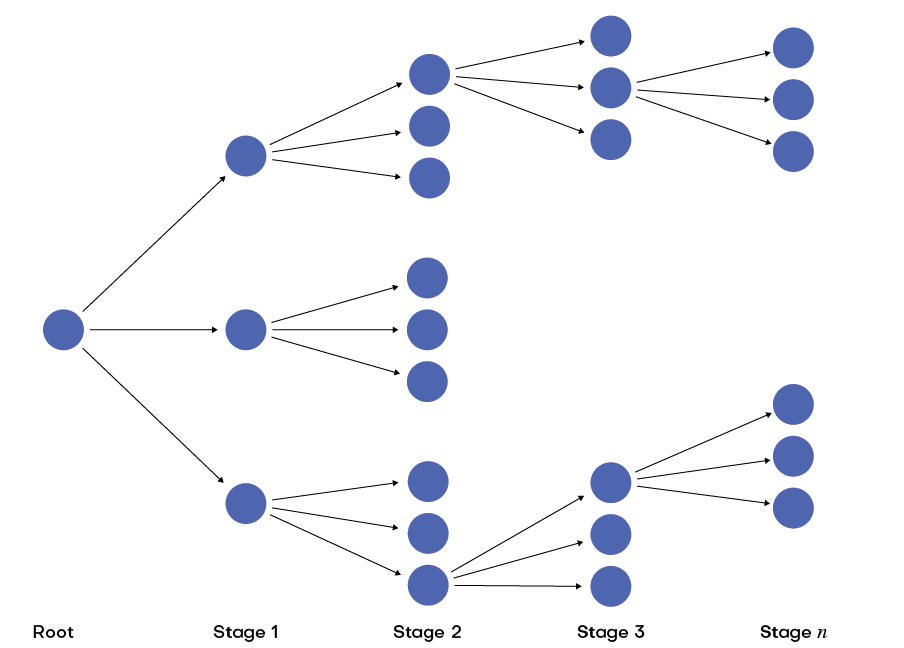
Figure 1: Multi-stage dimensionality issue
PLEXOS offers a scenario-reduction technique called “hanging branches,” which is described in the following section.
Hanging Branches Representation
Assuming we have a multi-stage stochastic problem consisting of four stages and three branches per stage, we can represent the tree as shown in Figure 2.

Figure 2: Full multi-stage tree for 4 stages and 3 branches per stage. 3 4= 81 scenarios to explore.
We can reduce this full tree to solve an equivalent multi-stage problem. There are several ways to reduce the stochastic tree: in this paper we reduce the stochastic tree by organizing the branches as “full branches,” “hanging branches” or “death branches,” which are defined as:
- Full branch: Path to be explored.
- Hanging branch: Uncertainty associated to the full branch to be explored.
- Death branch: Path to be discarded to avoid dimensionality issues.
If the user reduces the tree in Figure 2, to in three full branches and two hanging branches per stage, Figure 3 is the resulting tree.

Figure 3: Full tree classified in full, hanging and death branches
By deleting the death branches from the tree in Figure 3, we have the following reduced tree:
INDEPENDENCY
It is important to note that the inflows at the beginning of each stage are known. This means we can solve each full branch independently, as shown in Figure 5.
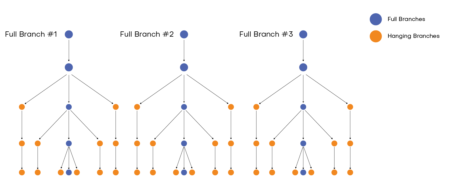
Figure 5: Resulting tree after assuming inflows are known at the beginning of each stage.
Hanging Branches Reduction
By default, the weights for each branch are uniform. In order to avoid dimensionality issues in the number of hanging branches, the user can set the weights used in the objective function for those branches.
We developed a sample reduction algorithm for hanging branches to reduce the number of samples to a predefined smaller number, but the reduced samples are still a good approximation of the original problem. The reduction is based on rules that ensure only the samples that are similar to other samples or have small probabilities are combined. The methodology is illustrated in the following figure:

Figure 6: Hanging branches reduction from 6 to 2 hanging branches per stage.
Rolling Horizon
To solve the resulting tree shown in Figure 5, PLEXOS offers a methodology called “rolling horizon.”
We represent one single, full branch of Figure 5 as follows when solving from a root node:

Figure 7: One single full branch with uncertainty at each stage.
The rolling horizon approach is designed to overcome the limitations of extremely small probabilities deep into the future. The method looks ahead to a given point in the future; the end volumes at that point are passed as initial volumes at the start of the next step.
For a horizon divided in multi-step stochastics, the algorithm works as follows:
Step 1:
- Starting date is beginning of root node.
- Multi-stage tree formulated from start to a user-defined stage in the future where no more branches will be added to avoid weights issue.

First roll:
- Starting date is beginning of stage 1.
- End volumes in first solve are passed as initial volumes in roll 1.
- The past branches are not formulated because that part of the problem is already solved.
- More hanging branches are formulated when the weights provide information to the optimization solver.

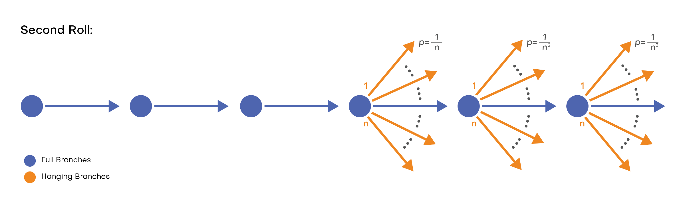
Second roll:
- Starting date is beginning of stage 2.
- End volumes in first roll are passed as initial volumes in roll 2.
- The past branches are not formulated because that part of the problem is already solved.
- More hanging branches are formulated when the weights provide information to the optimization solver.
The problem continues rolling until it has fully explored the horizon.
Rolling Horizons
Synthetic Sample Generation
Multi-stage stochastic optimization needs a large number of scenarios, or samples, to represent the equivalent tree. The literature includes different methods for creating these samples, however the simplest method creates future samples based on history.
If we have historical records from 2000 to 2011, and the user wants to create samples from 2019 to 2030, the we need to generate the number of full branches as described in the following table:
Table:2 Historical Information
| Simulated Year |
||||||||
| 2019 | 2020 | 2021 | ... | 2028 | 2029 | 2030 | ||
| Full Branches | 1 | 2000 | 2001 | 2002 | ... | 2009 | 2010 | 2011 |
| 2 | 2001 | 2002 | 2003 | ... | 2010 | 2010 | 2000 | |
| 3 | 2002 | 2003 | 2004 | ... | 2011 | 2000 | 2001 | |
| ... | ... | ... | ... | ... | ... | ... | ... | |
| ... | ... | ... | ... | ... | ... | ... | ... | |
| 12 | 2011 | 2000 | 2001 | ... | 2008 | 2009 | 2010 | |
| ... | ... | ... | ... | ... | ... | ... | ... | |
This method is powerful and simple, as it preserves the spatial correlation between hydro storages and doesn’t require statistical analysis.
To generate the hanging branches, we can use the historical information as well. For this purpose, the sampling method selects a different year for the same position in time.
A weekly multi-stage problem starting from historical year 2000 could look as follows:
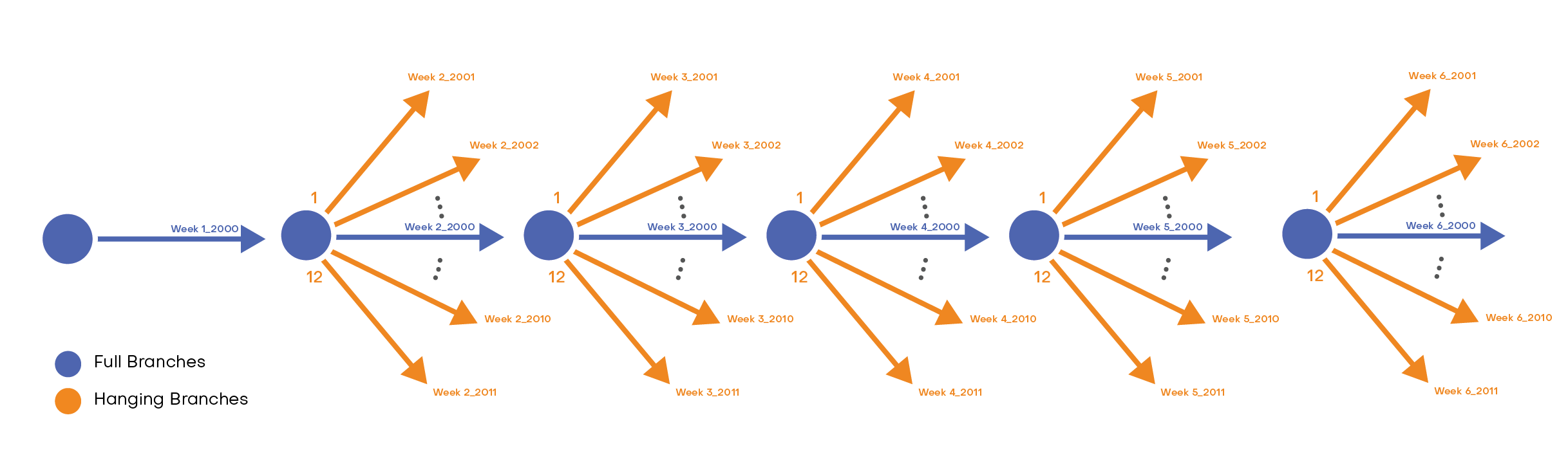
The hanging branches for full branch number 1 looks as follows: